poles and zeros of Laplace transform

[PG1995]

Thank you, Steve, nsaspook.

nsaspook: The document is good and thanks for sharing it. I need to read it carefully.

Regards
PG

 

[MrAl]

Hi

I'm still struggling with the interpretation of poles and zeros. How mathematical poles and zeros affect real circuits. I thought that to start with a series RC circuit would be a good idea.

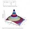
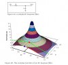
The following transfer functions are for a series RC circuit. The first one is for the voltage across capacitor and the second one is for voltage across resistor.

[latex]H_{C}(s)=\frac{1}{1+RCs}[/latex]
[latex]H_{R}(s)=\frac{RCs}{1+RCs}[/latex]

Both transfer functions have a pole at s=-1/RC where s=σ+jw. For transfer function Hr(s) zero exists at the origin.

What do pole and zero represent in this case? The cutoff frequency for a series RC circuit is [latex]w_{c}=1/RC[/latex]

Thank you.

Regards
PG

Note to self: The content from post #2 is relevant here.

Hello,

[Note that since the original post i had to correct a few typos here.]

The s plane has two axises, the real axis (along the normal x axis) and the jw axis (along the normal y axis).
If you plot the poles and zeros on this plane and pick a particular frequency w, you can then draw arrows from each pole and zero to the test frequency on the jw axis, where each arrow has a particular length and angle. The magnitude of the response is then the quotient of the product of the lengths of the arrows from zeros divided by the product of the lengths of the arrows from the poles, and the phase angle response is then all of the zero arrow angles minus all of the pole arrow angles.
For example for (s+2)/(s+3) we would plot one zero at (-2,0) the real axis and one pole at (-3,0) also on the real axis. Then for a test frequency of w=3 we would draw an arrow from (-2,0) to jw=3 which is at point (0,3) on the graph and that is the arrow for that one zero, then draw another arrow from (-3,0) to (0,3) and that is the arrow for that one pole. Now if the length of the arrow for the zero is Lz and the length for the pole Lp, and the angle for the zero is Az and the angle for the pole is Ap, the response magnitude is Lz/Lp and the phase angle is Az-Ap.
If there were more than one arrow for each then for the magnitude we would calculate the product of all Lz divided by the product of all Lp, and to get the phase angle calculate the difference of the sum of all Az minus the sum of all Ap.
In our above example the test frequency was w=3, so these calculations would produce the results for w=3. If we instead want to test at w=4, then we have to draw all the arrows over again and recalculate the lengths and angles, but that's how the poles and zeros affect the magnitude and phase angle responses.
For our example with a zero at -2 and pole at -3 and test frequency w=3, we have lengths:
Lz=sqrt(2^2+3^2)
Lp=sqrt(3^2+3^2)
and angles:
Az=atan2(3,2)
Ap=atan2(3,3)

so the magnitude response is sqrt(13)/sqrt(18) which is about 0.85 and the phase angle response is atan2(3,2)-atan2(3,3)=atan(3/2)-pi/4 which is about 11.3 degrees.
Note that if we changed the test frequency to w=4 we'd have to redraw the arrows and that would mean all the lengths and angles change slightly:
Magnitude=sqrt(2^2+4^2)/sqrt(3^2+4^2)=approximately 0.894
Phase=atan2(4,2)-atan2(4,3)=approximately 10.3 degrees

Attached is a diagram of s plane root locations and time domain response shapes.

 

[PG1995]

Thank you, MrAl.

I think at this stage it would be better for me to restrict myself to a series RC circuit because it would be comparatively easier to understand it. The document linked by nsaspook is quite helpful in this regards, especially the plot.

So far, this is what I have concluded. Laplace transform embeds information about frequency response and transient response of a circuit. Further, it also indicates troublesome points using poles and zeros which in turn help to analyze the stability of a system.

Q1:
What is the dimension of "s" in Laplace transform? I believe that it has dimensions of sec^-1. It further means that "σ" also has dimensions of sec^-1 and so does "w". Do I have it correct?

Q2:
a: The following transfer function has a single pole at s=σ+jw=-1/RC. It means that σ=-1/RC and jw=0. Do I have it correct?
b: Was this plot (source) drawn assuming some specific values for "R" and "C"? I'm saying so because from the plot it looks like the pole (i.e. the response going infinite) occurs between σ=-1.5 and σ=-2 and jw=0. What do you say?

[latex]H_{C}(s)=\frac{1}{1+RCs}[/latex]
Q3:
In this plot you can see that when jw=0 (i.e. DC signal) and σ=0, the normalized response is 1 or 0 dB (the blue dot). But as σ<0, say -0.5, the response becomes, say 3. The jw is still "0" which means DC signal.

What does σ<0 mean in this case? Does it have anything to do with values of resistor and capacitor? I don't see how. If Vin=5V then I don't think changing the values of either resistor or capacitor would change the output voltage across capacitor; the output voltage would still be 5V.

Q4:
I have googled to find out an easy way to plot 3D surface of a transfer function. I found this page. I downloaded the file from this page but getting the following error:
Error in ==> s_plane at 6
syms s unreal % making (s) as a symbol

My Matlab version is 7.12.0.635 (R2011a).

Could you please help me with the queries above? Thank you.

Regards
PG

Helpful link(s):
1: http://www.chem.mtu.edu/~tbco/cm416/PolesAndZeros.html

 

[MrAl]

Hi

[1]
w is in radians per second, lower case sigma is in nepers per second.
s is whatever you make it.

[2]
That plot looks like it was made for a normalized RC time constant, therefore when lower case sigma=-1/RC we get an infinite response.

[3]
Lower case sigma would be part of the drive signal.

[4]
Dont have it, sorry, maybe someone else here can help with this.

 

[PG1995]

Thank you, MrAl.

Let's proceed slowly so that I don't make it any more messy.

[1]
w is in radians per second, lower case sigma is in nepers per second.
s is whatever you make it.

In my humble opinion, I think that "s" should have unit of sec^-1 because then the expression e^(s*t) would be unit-less. In order for the "s" to be dimensionless, don't you think that "w" and "σ" should have similar units?

[2]
That plot looks like it was made for a normalized RC time constant, therefore when lower case sigma=-1/RC we get an infinite response.

How would define this "normalized RC time constant"?

If you read the topic "First-Order Filters" at the top in this document, it says:

"An integrator (Figure 1a) is the simplest filter mathematically, and it forms the building block for most modern integrated filters. Consider what we know intuitively about an integrator. If you apply a DC signal at the input (i.e., zero frequency), the output will describe a linear ramp that grows in amplitude until limited by the power supplies. Ignoring that limitation, the response of an integrator at zero frequency is infinite, which means that it has a pole at zero frequency. (A pole exists at any frequency for which the transfer function's value becomes infinite.)"

I understand the infinite response notion in this context of integrator but couldn't mentally picture such an infinite response in case of a series RC circuit. I believe that in case of a RC circuit, infinite response would mean a very large voltage across capacitor. Could you please help?

[3]
Lower case sigma would be part of the drive signal.

Okay. So, "jw" represents sinusoid drive signal and σ also represents a drive signal but I suspect it's a decaying exponential drive signal.

Thank you.

Regards
PG

 

[MrAl]

Hi again,

Well w is angular frequency and is equal to 2*pi*f, and since f=1/t then you could look at it as 2*pi/sec i guess, so it is scaled frequency or scaled inverse time. Officially it is radians per second.
Lower case sigma officially is in nepers per second.
I think more officially too s is in units of "complex nepers per second".
You could probably look up 'neper' and see what you can make out of it.

When we normalize something, we call that something 1. So if the plot is normalized to -1/RC, then when lower case sigma is equal to -1/RC we look at the place where sigma is equal to -1. If you like, you can just call RC=1 (the produce of R and C is 1), and that produces a specific case.

Yes i believe sigma is the exponential, either positive or negative.
For the RC filter, we have transfer function:
1/(s*R*C+1), or dividing top and bottom by 1/RC we have:
(1/RC)/(s+1/RC)

and if we call 1/RC just 'A' such that A=1/RC then we have:
A/(s+A)

Now for a sinusoidal signal we can set s=jw as i am sure you have seen many times. This gives us a complex transfer function:
A/(jw+A)

and we can vary w to find the response to various angular frequencies.

But what if we set s equal to jw+a, where a=sigma here, we now have:
A/(jw+a+A)

The plot shows that the angular frequency is zero, so this means w=0 so we have:
A/(0+a+A)

or just:
A/(a+A)

Now if we look at this we can see that if a=-A, we'll get an infinite response.
Since A=1/RC that means that if a=-1/RC then the response goes infinite. This is interesting because the time solution doesnt seem to go infinite but seems bounded.

You might also look at e^(s*t) where s is complex again: s=jw+a, where a can be plus or minus.

 

[steveB]

PG,

Radians, nepers and cycles are all dimensionless units. Hence rad/s, nepers/s, Hz, cycles/s or 1/s are all the same units of inverse seconds. The purpose of using the dimensionless units is to make it clear what context the unit is used in. Nepers is always used with an real exponential (not complex or imaginary), while radians is always used with a sinusoidal function. The s represents a complex frequency with units of inverse seconds. While the sigma has units of nepers/s and the w has units of rad/s, it is better not to assign either name to s itself. Just call it a frequency or complex frequency with units of inverse time and typically inverse seconds in practice.

Also, as I pointed out before, you can't see the infinity unless the pole is on the jw axis. In other words the pole would have no real part and then you would see the Bode plot blow up. If your pole/zero plot represents a real system, then the thing that will blow up is the ratio of output over the input. There will be regions of convergence in the s-plane and their will be poles and zeros that are relevant.

I can't stress enough the need to work with systems and control theory directly, either as real world problems or text book problems. You've asked these same questions many times in the past, and my theory is that it is not sinking in because you expect that answers given in a vacuum will be completely understandable. Electrical engineers understand this stuff better than any other profession because we work with it to solve real problems. I've never met a mathematician, physicist or theoretician that has any where near a good understanding of the "meaning' of poles", as do practicing engineers that use this stuff to put food on the table. Ive also never seen an electrical engineer give a good explanation of the "meaning of poles" either, despite their very good understanding. I don't mean that their answers are bad, but their answers never have the power to make the "uninitiated" truly understand the intricacies involves.

Here is a simple problem for you to try. Make a Simulink model of a simple RC circuit and then start feeding various decaying sinusoids into the system and look at the output. Then plot the output over the input and observe what happens if you are not in a region of convergence, if you are in a region of convergence, if you are at a zero, or if you are at a pole. If you try this, you will gain true insight, and if anything about this confuses you , then ask direct questions here and show us plots of your simulations. This will be far more productive than pecking around the question with abstract answers.

 

[MrAl]

Hi,

The poles and zeros to me are the anchor points of the vectors i had shown in a previous post as arrows. This is the most geometrically solid explanation i think.

We have to be careful what we call these quantities, like w and sigma. Hertz is a unit of frequency which is equal to cycles/second. In one cycle there are 2pi radians, so w has to be in radians per second, strictly speaking. If we dont do this, then the context has to be explicitly clear.
For example, if i say i have a filter that has cutoff of 12.5 Hertz then we have to take that to mean frequency in cycles per second unless the context has made it clear that we are talking about radians per second (w). So i like to look at w as being in units of scaled frequency, or scaled inverse seconds, where the scaling factor is 2*pi.
Likewise if i measure the length of a drill shank and say that it measures "5 inches", then i can not mean that it is really 2*pi*5 inches.

The neper refers to a scale that has a logarithmic nature, after the inventor.

For some reason they sometimes refer to 's' itself as being in units of "complex nepers per second". This might be because the sigma part is the 'real' part, and we often refer to quantities based on their real part as being the most important part.
I have always called it "complex frequency" however, because that is the more typical use of the variable s, and they are both frequencies.
The two names apparently come from taking the name from either the imaginary part as the more important view or the real part as the more important view.
For example, if s=j*w+0 then it is more of a frequency, but if s=0+sigma then it is more of a neper per second quantity. Perhaps a better name would be "frequers" (ha ha), or "nepency" (ha ha).

 

[PG1995]

Thank you, Steve, MrAl.

Although this time I don't think that I was being completely vague with this topic, we were discussing series RC circuit using a 3D plot of it which shows its gain against complex variable "s". Anyway, as you already know that I don't know how to use Simulink therefore I have decided to start learning it. Thank you.

Regards
PG

Helpful link:
Explanation of Neper (source)

 

[steveB]

Although this time I don't think that I was being completely vague with this topic, we were discussing series RC circuit using a 3D plot of it which shows its gain against complex variable "s".

Not sure what you are trying to say here. Your question was not vague at all, and yes we did discuss that.

Anyway, as you already know that I don't know how to use Simulink therefore I have decided to start learning it.

Actually I don't know that you dont know how to use it. Other times you mentioned you were going to learn it, so I just assumed you knew it at least a little bit by now. Anyway, this is a good example of why I say it is time to get to work. It does not take much time to learn the basics of Simulink, and if it does it is because you dont have someone to run through the basics quickly to speed up the process. A first order system is the simplest example you could try, so it seems like a good place to start.

 

[MrAl]

Hello again,

I probably forgot the basic mechanism behind using the exponential drive signal because it's been a long time since i had looked at that. When i do it today in the time domain, i dont get an infinite response, but i do get an infinite response when i plug it into the frequency domain equation.
It's not that hard to create an exponential source. All i had to do was use a general purpose source and declare that the voltage would be:
v=e^(-t)
and that creates a decreasing exponential.
As we might have guessed, when driving an RC filter (low pass) with this drive signal it does not generate an infinite response. To check, doing a more direct time domain analysis results in the same thing.
Interesting though is that the denominators of the analytical form approach zero, but because the limit also depends on the numerators and one numerator has e^-t in it, we end up with a 'bump' waveshape in time, which goes to zero as time progresses. So it seems bounded.
Perhaps there are just some things that we just dont do, but there should be a reason behind why we dont do it if we really dont do it. Perhaps it is just not the same thing exactly, or perhaps the frequency domain solution is just telling us something more abstract.
If we draw arrows from the pole to the jw axis we can determine the frequency response. But if we try to draw arrows from the pole to the real axis, we end up with an arrow that starts at -1/RC and ends at -1/RC which means the length of one arrow is 0.

 

[steveB]

Hello again,

I probably forgot the basic mechanism behind using the exponential drive signal because it's been a long time since i had looked at that. When i do it today in the time domain, i dont get an infinite response, but i do get an infinite response when i plug it into the frequency domain equation.
It's not that hard to create an exponential source. All i had to do was use a general purpose source and declare that the voltage would be:
v=e^(-t)
and that creates a decreasing exponential.
As we might have guessed, when driving an RC filter (low pass) with this drive signal it does not generate an infinite response. To check, doing a more direct time domain analysis results in the same thing.
Interesting though is that the denominators of the analytical form approach zero, but because the limit also depends on the numerators and one numerator has e^-t in it, we end up with a 'bump' waveshape in time, which goes to zero as time progresses. So it seems bounded.
Perhaps there are just some things that we just dont do, but there should be a reason behind why we dont do it if we really dont do it. Perhaps it is just not the same thing exactly, or perhaps the frequency domain solution is just telling us something more abstract.
If we draw arrows from the pole to the jw axis we can determine the frequency response. But if we try to draw arrows from the pole to the real axis, we end up with an arrow that starts at -1/RC and ends at -1/RC which means the length of one arrow is 0.

To see the pole blow up, we need to take the ratio of output over input and take the limit as time goes to infinity. This is not quite a proper thing to do in the general case of complex poles, but it works for real poles and for exponential inputs.

If we have a transfer function of T=1/(s+1), and we put in exp(-t) then we are at a pole and the ratio of output over input is a straight line which goes to infinity.

Now put in exp(-t/2) and the output will asymptotically approach 2, as expected from the transfer function.

Here is the tricky part. Put in exp(-2t) and the ratio diverges even though we are not at the pole. The reason is that now the input in not in the region of convergence (ROC) for the single sided Laplace transform.

For pure sinusoidal inputs (jw axis), you cant divide output over input in the time domain, but you can compare amplitude and phase easily and then take the ratio in the frequency domain. For example consider w=1 for poles at +i and -i . The response is 0.707 at a phase of 45 degrees and this can be seen in the time domain.

For complex pole locations, or complex input locations, then you have to be more careful when comparing the input and output in the time domain. You need to look at both amplitude and phase and it is not usually easy to see the answer if the real and imaginary parts are of the same order or magnitude.

This is exactly why I recommend that PG try these things himself. Only by experimenting and seeing the results and by trying to understand and interpret the answers can we truly understand the meaning of the abstract theory.

 

[MrAl]

Hi again,

Very nice Steve, and i'll have to read this again and try to remember how to make sense of that aspect of it. This is something that almost never comes up in practice so it was probably 30 years ago the last time i saw anything like this, or needed to.

 

[PG1995]

Thank you, Steve.

Actually I don't know that you dont know how to use it. Other times you mentioned you were going to learn it, so I just assumed you knew it at least a little bit by now.

Yes, you are right in saying that I mentioned in the past that I was going to learn Simulink. I'm sorry but I never did. I think that the best platform for a student to learn such stuff is a school where someone sitting next to you can easily guide you. Unfortunately, in my school they never made us learn it.

Anyway, this is a good example of why I say it is time to get to work. It does not take much time to learn the basics of Simulink, and if it does it is because you dont have someone to run through the basics quickly to speed up the process. A first order system is the simplest example you could try, so it seems like a good place to start.

Yes, this is what I had thought and that's why I have already created a new thread about it a day ago. I believe that not many persons on this forum use Simulink or it's just that they find it hard to help someone with this stuff on a forum. Anyway, I have started learning it. Thank you.

Regards
PG

 

[steveB]

Yes, you are right in saying that I mentioned in the past that I was going to learn Simulink. I'm sorry but I never did. I think that the best platform for a student to learn such stuff is a school where someone sitting next to you can easily guide you. Unfortunately, in my school they never made us learn it.

No need to apologize. It's your choice where you place your priorities. I'm just stressing that if these types of questions are a priority for you, then it will be more time efficient to learn tools like Matlab and Simulink to help get insight faster and to get a viewpoint that is more intuitive. These are the tools of the trade, so to speak.

Definitely it is better to have someone right there to help you, but if you don't have that, then try tutorials and online videos etc. I've attached a Simulink file which has some of the pieces needed for this.

 

[PG1995]

Thank you, Steve.

If we have a transfer function of T=1/(s+1), and we put in exp(-t) then we are at a pole and the ratio of output over input is a straight line which goes to infinity.

I'm sorry but I don't really get it. Transfer function is 1/(s+1) and Laplace transform of exp(-t) is 1/(s-1). How are your manipulating the expressions so that the ratio of output over input is a straight line which goes to infinity?

I'm just stressing that if these types of questions are a priority for you, then it will be more time efficient to learn tools like Matlab and Simulink to help get insight faster and to get a viewpoint that is more intuitive. These are the tools of the trade, so to speak.

I always value your advice and I have noticed over years that what you say mostly proves to be true. In the future I will try to focus on Matlab and Simulink.

The Simulink file attached by you uses .slx extension and it cannot be opened in R2011a Matlab being used by me. Could you please save your .slx file into older .mdl extension and attach it here? By the way, I also tried to design a Simulink model of RC circuit here. Thank you.

Regards
PG

 

[steveB]

I've attached a .mdl file for you. The way you are making the system looks correct, but I prefer to use the transfer function block as I show in my file.

You will see in my model that I simply take the output divided by the input. As I mentioned above, this is generally not the right thing to do. We take ratios in the frequency domain, not the time domain, but for exponentials, there is no phase to worry about so the ratio, taken to t=infinity, allows the initial transients to die off, and allows the steady state ratio of amplitudes to be measured.

 

[steveB]

Another aspect of this is to understand "regions of convergence". When we look at poles and zeros, we are not completely specifying the signals. The region of convergence is the missing piece of the puzzle. Typically in real problems we deal with the single-sided Laplace transform which assumes signals are zero for t<0. In other words all signals are multiplied by u(t), the step function.

You need to watch and understand the following lecture.

 

[Tony Stewart]

For more complex systems they use better methods such as Root Locus stability criteria, which I leave for your homework.

 

[MrAl]

Hi,

Yes i have found the Root Locus procedure to be the most useful of all. There are even some programs that will graph it for you given the transfer function.

But there is a practical consideration to this too and that comes about because we are dealing with real valued components that change over time and temperature and sometimes even a small change can make a big difference. Let me give a very simple example...

First we have Ts=1/(s-a) with positive 'a', and the step response to this is e^(a*t)/a-1/a which we can see is an ever increasing exponential.
So if we add (s-a) in the numerator and get:
Ts=(s-a)/(s-a)

and the inverse transform of the step response for this is just 1 which is completely stable. But that only works if the numerator was the consequence of an algebraic operation because although 'a' is a constant here theoretically, in practice it is only a constant when the numerator resulted from some calculation that gave us the derivation of that numerator, not some separate physical entity. For a separate physical entity, we have to think like this instead:
Ts=(s-b)/(s-a)

where b=a, and again in theory that still results in a step response inverse transform of 1, but in practice 'a' might be 1/(R1C1) and 'b' might be 1/(R2C2), and if R1C1 is not equal exactly to R2C2 for every possible environmental extreme, we could end up with a very unstable system. So just because 'b' was set equal to 'a' by design, that doesnt mean it will be stable forever in a real life design.