Electro Tech is an online community (with over 170,000 members) who enjoy talking about and building electronic circuits, projects and gadgets. To participate you need to register. Registration is free. Click here to register now.
Welcome to our site! Electro Tech is an online community (with over 170,000 members) who enjoy talking about and building electronic circuits, projects and gadgets. To participate you need to register. Registration is free. Click here to register now.
Because right plane poles come from regenerative feedback. Have you had control theory? Have you taken differential equations? The reason I ask is so that I don't want to give a mathematical answer you might not understand.
Hello Ritesh .. In the time BrownOut gets back to you,,
To clarify things, we must specify that when we say "right half plane" is unstable and "left half plane is stable", we're talking in s plane. If you want the z plane thing, feel free.
To get the left half plane "thingy", we must go back to constant coefficients differential equations and solving them with a characteristic equation. Second order, for example...
y'=dy/dt and y''=d2y/dt2 (I'm on a MacBook, don't hold typos on me)
Homogen equation (second part null)
a*y'' + b*y' + c*y = 0
We arrange a bit to make it look like : y'' + 2*Ksi*w*y' + w^2*y = 0 ..
Where Ksi is the damping coefficient, and w is omega, the natural pulsation of the system. (Hint : w^2= c/a... So Ksi is ?)
We look for a solution of the exponential form .. e^(s*t)
Characteristic equation of the differential equation above becomes : s^2 + 2*Ksi*w*s + w^2=0
Simple second degree. You find Delta' (Simplified Delta, we arranged the two so you don't get a 4, and you don't divide by 2)
Solutions will depend on the value of Ksi..
Ksi Superior to 1 (Delta Positive) : Two Simple (non double) Real solutions , e^(s1*t) and e^(s2*t)
Ksi = 1 (Delta Null) : The solution is double and real (A*t + B)*e^(s*t)
Ksi Inferior to 1 (Delta Negative) : Imaginary solution (two conjugates) ... s here is : s=u + i*v (i^2=-1)
First solution is (e^(u*t))*(Cos(v*t) + i*Sin(v*t)) (t being the time, v the imaginary part of s, and u the real part of s)
WHAT DOES ALL OF THIS MEAN ?
Notice that the Amplitude of these solutions DEPENDS on the REAL value of the solution.( The first and second cases where Delta is positive or null, s is real, so s=u.. No imaginary part)
They are exponential type. So, it's e^(u*t).
If u is positive, amplitude grows exponentially. And in the case of the imaginary solution, it's a sinusoide with an exponentially growing amplitude.. You don't want a system like that. It's a DIVERGENT system. Unstable.
If u is negative thought, amplitude gets "damped" with respect to time. It's a CONVERGENT system. Stable.
Hi, I'm sorry I let this slide. I didn't want to get into alot of math, because I knew that would just lead to more and more questions. I wanted to write something intuitive, but I blew it. I have alot on my plate. I'll try to put something together soon.
Ksi is the damping coefficient. We're not "using" Ksi, or "w"... We're just making them "shine".
It's better to write s^2 + 2*Ksi*w*s + w^2=0 than to write a*s^2 + b*s + c=0. It's the EXACT SAME equation.
So why are we doing it ? Well, for practical reasons.Imagine I tell you to simulate a system with a natural pulsation of 2 rd/s and a damping coefficient of 0.7.. To do that in the second equation, you would have to JUGGLE with a, b and c to get those two values. Whereas in the first equation, you just assign Ksi and w 0.7 and 2 rd/s respectively and simulate.
Arranging the equation to make it "look" a certain way, to make the damping coefficient and the natural pulsation appear as parameters is just more practical and gives you more information in one glance.. If I give you a system with an equation like s^2 + 2*0.8*2*s + 4=0, you immediately KNOW that the damping is 0.8 and the pulsation is 2rd/s .. It just JUMPS at you. Try doing that with the raw characteristic equation.
The most known, most used, actually the first name that any Teacher in any University of any country I think will mention in the very first class of any Control Theory course in the World, is MATLAB.
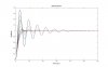
In the attachement, I simulated the step response (a response to a Heaviside step) for different values of damping, from .1 to 1 (From pseudo-periodic to critic, I didn't do the a-periodic when Ksi>1)
It helps to look at a very simple system with feedback that is known to oscillate with some value of the forward section gain.
In the attachment, we make all the resistors equal to 1 ohm and all the capacitors equal to 1 Farad for simplicity.
Evaluating the circuit, we get for the forward section:
G=gain of upper amplifier=G
and in the feedback section we get:
H=1/(s*R*C+1)^3
Thus the equation we use for the roots is:
1+G*H=(s^3*C^3*R^3+3*s^2*C^2*R^2+3*s*C*R+G+1)/(s*C*R+1)^3
Setting this equal to zero, we get:
(s^3*C^3*R^3+3*s^2*C^2*R^2+3*s*C*R+G+1)=0
This is the equation we solve to find the roots.
Since R=1 and C=1, we have:
s^3+3*s^2+3*s+G+1=0
which is a fairly simple third degree equation in the variable 's'.
Now we vary the gain G to see what effect it has on the roots.
Looking at the roots with G=0, we get three roots:
s=+0*j-1
s=-0*j-1
s=-1
Examining the real part of all three roots, we see that all of
the real parts are less than zero. This puts all the poles
in the left half plane so the system is stable.
Now we look at the roots with G=5, we get three approximate roots:
s=+1.48088*j-0.145012
s=-1.48088*j-0.145012
s=-2.7099759
Looking at the real parts of these three roots, we see that the
first two roots have migrated closer to zero so the system is
starting to become less stable. They are all still in the left
half plane so it is considered stable.
Now we look at the roots with G=7.9, we get three approximate roots:
s=+1.724803*j-0.004185
s=-1.724804*j-0.004185
s=-2.991632
Looking at the real parts of these roots now, we see that the
first two have gone down to very close to zero. The system is now
almost an oscillator.
Now lets look at the roots with G=8.1, we get roots:
s=+1.739237*j+0.004149
s=-1.739238*j+0.004149
s=-3.008299
Now we see that the real parts of the first two roots have moved into
the right half plane. The circuit is now an oscillator that may saturate
after some time.
With G=10 we get approximate roots:
s=+1.865795*j+0.077217
s=-1.865796*j+0.077217
s=-3.154435
and we see that the roots are moving farther into the right half plane.
With G=100 we get approximate roots:
s=+4.019733*j+1.320794
s=-4.019734*j+1.320794
s=-5.641589
and we see that the real parts of the first two roots moved even farther into the right half plane so the circuit is unstable.
In the diagram below we have the circuit and under that the pole constellation diagram drawn on the complex plane.
The red circles are for the sets of roots that dont have any part in the right half plane, while the orange dots are for the sets of roots that do have some roots in the right half plane.
Looking at the roots that are drawn as red circles, they are all in the left half plane.
Looking at the roots drawn as orange dots, two of the roots of those sets are in the right half plane.
There are no zeros in the transfer function so there are no zeros to consider.
In fig. the top most op-amp is used at a gain of 7.9, why you have taken 7.9 or any other value ...??
and then output of amplifier is feed to in put by using low pass filter then buffering signal with buffer ( of gain 1)..3 low pass filter are used like phase shift oscillator, acting as phase delay... I am right??
We get H like that because that's what we get when we analyze the bottom section of the circuit from output back to input.
Im sorry, it's supposed to be typed as 1/(s*R*C+1), my mistake in typing. It's fixed now.
I took 7.9 for example because i knew beforehand that 8.0 was an important value for the gain G because that's when the roots cross the imaginary axis and the circuit becomes unstable.
I took G=0 because that's a good place to start the root determinations. Then, i let G grow larger and larger too see if any roots crossed over into the right half plane. I saw that as G got larger two of the roots moved closer to the j axis and then finally when G>8 they moved right into the right half plane so the circuit became unstable.
Yes this circuit could be a phase shift oscillator, but only with the right value of gain G. It wont oscillate unless the gain is at least 8. That's one of the things we like to determine when doing this kind of analysis.
When the gain is less than 8 the circuit is damped so it doesnt oscillate (stable). When the gain is 8 it oscillates (conditionally stable), and when the gain is greater than 8 it oscillates for a while and then saturates the system (unstable).
This site uses cookies to help personalise content, tailor your experience and to keep you logged in if you register.
By continuing to use this site, you are consenting to our use of cookies.