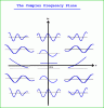
How do I visualize this, s, complex angular frequency? Kindly help me.
With various transforms, you can imagine that you are applying a particular "test" function to a system. When we use Fourier Transforms, we can imagine that we are applying sine and cosine waves (or complex exponentials) to the system, and we look at how a system responds to that input signal. Laplace Transforms are one step more general than Fourier transforms because you get the Fourier Transform when σ=0.
So, imagine that you are applying signals of the type exp(-σt) sin(ωt) u(t) or exp(-σt) exp(jtω) u(t). In other words, imagine a decaying sine wave for starters. Now, the class of test signals is more general than this because you can have pure sine waves, pure decaying exponentials, exploding exponentials and increasing sine waves etc.
In essence, the σ is a decay (or expand) rate (units of 1/sec are sometimes called rates), and ω is a frequency (units of 1/sec are also sometimes called frequencies). The two are combined and called a complex frequency traditionally, but don't let the word frequency throw you off what the concept is.
I'm not still clear about
the Q2. Could you please help me with it?
I think MrAl hit the nail on the head when he mentioned the impulse function. The Laplace transform is an integral and impulses are objects that generate non-zero numbers when integrated. If you start your integration at 0+, you miss the contribution of the impulse function.
Keep in mind that some systems depend, not only on the input signal, but also on derivatives of the input signal. Hence, even responses to step functions, ramps etc. have information in them from 0- to 0+ because derivatives generate impulses.
If it is still not clear, just be aware of the general importance of the distinction and then as you do more and more examples, it will become obvious.
If |exp(-σt)|=1 is incorrect, then what should it be? Please let me know. Thanks.
I guess it should be |exp(-σt)| is equal to 1 if σ equals zero and |exp(-σt)| not equal to 1 if σ is not equal to zero. The σ is a parameter that can take on any real value.

")