Audio Transformers and Two-ports

[The Electrician]

Audio transformers seem to often raise the question of what is the impedance rating of the various windings, and what determines those impedances? How can we measure the rated impedances?

Discussion of the impedance transforming properties of transformers can be found in many textbooks and many web sites, but I'll review certain aspects of those properties especially contrasting the differences between the behavior of ideal transformers compared to the behavior of real transformers.

Let's only consider a transformer with two windings, an audio output transformer with a relatively high impedance rated primary and low impedance rated secondary. If the transformer were ideal, it would have infinite inductance primary and secondary and no losses and no distributed capacitances causing self-resonances.

We could almost make such a thing if the windings were made or room temperature super conducting wire, and if the core material were magnetic unobtainium having infinite permeability and no hysteresis or eddy current losses. We would still have distributed capacitances, though, but I'll ignore the losses from real dielectrics.

Suppose we wanted our transformer to have a 5000 ohm rated primary and 8 ohm rated secondary. Then we would need a turns ratio of 25 to 1; denote that as Nt and let the impedance ratio be Zt = Nt*Nt. We could wind the primary with 250 turns and the secondary with 10 turns (of superconducting wire).

When we discuss impedances connected to or measured at a winding, the measurement will be made with an AC signal of some moderate audio frequency, typically 1 kHz.

Now, we know that if we connect a load of RL ohms to the secondary and measure the impedance at the primary, we would expect to measure Zt*RL ohms. So, for a secondary load impedance of 8 ohms, we would measure 5000 ohms at the primary; for a secondary load of 80 ohms, we would measure 50,000 ohms at the primary. For a secondary load of .8 ohms, we would measure 500 ohms at the primary. This is all with the ideal transformer.

What if we connected a load impedance ZL of zero ohms (a short circuit) to the secondary? The expected primary impedance would be Zt*zero = zero ohms. A short on the secondary would be reflected as a short (zero ohms impedance) on the primary; remember, we are still talking about the behavior of an ideal transformer.

If we connect a load impedance of infinite ohms to the secondary, we would expect to measure Zt*? = ? ohms at the primary with the secondary open circuited. This is in accord with the infinite inductance our ideal transformer would have at both its windings.

So, we can expect that as the load impedance connected to the secondary ranges from zero ohms (a short) to ? ohms (open circuit), the primary impedance will also range from zero to ?. In other words, the primary impedance can have any value at all.

What about the behavior of a real transformer? Such a transformer will be wound with wire which is not super conducting, so it will have resistance. The core material won't have infinite permeability, so the winding inductances won't be infinite; the core material will have finite hysteresis and eddy current losses. The transformer model as presented in the transformer references I mentioned at the beginning will have a series resistance representing the copper losses, and a shunt resistance representing the core losses.

These losses will modify the impedances seen at the primary for various loadings on the secondary. For example, when the secondary has a zero ohms load (a short), the impedance seen at the primary will be increased by the resistance of the primary wire plus the reflected value of the secondary wire resistance; the primary impedance won't be zero ohms with a short on the secondary as it was with the ideal transformer.

When the load on the secondary is infinite ohms (open circuit), the primary impedance won't be ? because the equivalent shunt resistance representing the core loss will be in parallel with the reflected value of the infinite secondary load, giving a value just equal to the shunt equivalent of the core loss.

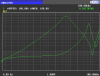
To see all this in action, I've taken a small output transformer with a 5k ohm rated primary impedance and an 8 ohms rated secondary impedance and measured the primary impedance with an open circuit on the secondary, and with a short on the secondary. The primary impedance magnitude was measured with an impedance analyzer from a low frequency of 4 Hz to a high frequency of 100 kHz. The impedance magnitudes are plotted on a log-log graph with 4 Hz at the left edge and 100 kHz at the right edge; major vertical lines are at 10 Hz, 100 Hz, 1 khz and 10 kHz. The impedance scale goes from 100 ohms at the bottom edge of the plot to 100k ohms at the top, with major horizontal lines at 1k and 10k ohms. This plot is shown in the attachment.

The top green curve is the primary impedance with the secondary open circuited (Zoc), and the bottom green curve is the primary impedance with the secondary shorted (Zsc).

The primary impedance can't be any greater than the top curve, no matter what impedance is connected to the secondary, and also can't be any less than the bottom curve no matter what impedance is connected to the secondary. In other words, the impedance we measure at the primary must always fall between the two green curves (up to 20 kHz or so), whatever resistive load we connect to the secondary (capacitive loads can cause the impedance to go a little above the upper green curve, but I'm not getting into that now).

We see that starting at the left side, the upper curve rises as frequency increases. This is because with the secondary open circuited, we are getting no transformer action, and we are just measuring the finite inductance of the primary, whose impedance increases with increasing frequency, as inductors do. Eventually we reach the self-resonance frequency of the primary at about 3 kHz, and then the open circuit impedance begins to decrease with increasing frequency, because the impedance is now capacitive. This is one of the limitations of a real transformer versus an ideal one.

The maximum impedance occurs at the first parallel resonance of the primary winding, but we see that there are more resonances at higher frequencies; for example, the first series resonance, giving an impedance minimum occurs at about 48 kHz.

The lower curve which is the primary impedance with the secondary shorted starts out at about 300 ohms at 4 Hz, and is nearly flat until about 1 kHz where it starts to rise due to the leakage inductance. We see a couple of resonances at higher frequencies. Since the secondary load impedance can't be less than zero ohms (we won't consider negative resistances), the primary impedance must always fall above the lower green curve up to about 20 kHz.

Unlike the ideal transformer which can be used with any value of secondary impedance, this real transformer can't have a primary impedance of greater than about 21k ohms at 1 kHz. This means that if we connected a secondary impedance of 64 ohms, the ideal transformer would transform that to a primary impedance of 40k ohms, but the real transformer just couldn't do that. The real transformer's primary impedance can't be more than about 21k ohms at 1 kHz; the real transformer's ability to transform impedances is limited by its losses.

This defect doesn't just kick in at a primary impedance of about 20k ohms; as soon as you move away from the optimum primary impedance of 5k ohms, the effect begins to occur. I'll discuss more in the next post.

 

[ericgibbs]

hi TE,
This pdf is also a useful reference for anyone interested in the Topic.
E.

https://www.google.co.uk/url?sa=t&r...2hEZWnvFg&sig2=l4vULNJRP4E-aohPYWTZcw&cad=rja

 

[duffy]

This is a fine explanation of why impedance is such a poor way to spec a transformer. Several times I've had to blindly purchase signal transformers and measure them to determine turns ratios, inductance and winding resistance. Incredibly, these things aren't listed in many spec sheets, and it's like a mechanical engineer being handed a drawing with floating dimensions.

 

[The Electrician]

Consideration of the properties of two-ports (https://en.wikipedia.org/wiki/Two-port_network) can lead to further understanding of the impedance properties of audio transformers.

A very simple two-port is the resistive attenuator in its several forms:
https://www.rfcafe.com/references/electrical/attenuators.htm

Any resistive network such as the resistive attenuator can serve as an impedance matching network between an input port and output port, albeit with attenuation. It is a property of networks like this that there is a pair of impedances (under almost all circumstances) that when connected to the the input and output ports, provide a simultaneous impedance match at those two ports. Those two impedances are called image impedances. They are usually designated Zi1 and Zi2. They are a property only of the two-port itself.

Zi1 is the input image impedance and Zi2 is the output image impedance. If Zi2 is connected as a load to the output of a two-port and the input impedance of the two-port is then calculated (or measured), that input impedance will be equal to Zi1. Similarly, if an impedance of Zi1 is connected to the input of the two-port, the impedance calculated (or measured) at the output of the two-port will be equal to Zi2.

When Zi1 is connected to the input of the two-port and Zi2 is connected to the output of the two-port, both ports are impedance matched, simultaneously.

How can we determine what the image impedances of a two-port are? In the case of a two-port composed of a network of known resistors, we can find the image impedances with arithmetic. We can also make use of a theorem known since the early days of Bell Labs.

Given a two port, measure the input impedance with the output port open-circuited; call that impedance Zoc. Then measure the input impedance with the output port short-circuited; call that impedance Zsc. Then Zi1 = SQRT(Zsc*Zoc); this value is the geometric mean of Zsc and Zoc. The same procedure can be followed to determine the output image impedance, Zi2.

This same procedure is well known as a method to determine the characteristic impedance of a transmission line. A length of transmission line is essentially a two-port; it has an input and output port.

An audio transformer is an electronic device that lends itself especially well to treatment as a two-port device. We can find the input image impedance and output image impedance of our output transformer and those impedances are the impedances which will provide a simultaneous impedance match at input and output. These impedances, in fact, should be very close to what the manufacturer specifies as the rated impedances of the windings.

An interesting propertry of logarithmic plots such as the one in the post #1 is that at a particular frequency, 1 kHz perhaps, if you read off the value from the top curve and from the bottom curve, multiply those values and take the square root of their product, that value, if then plotted on the same graph, will be a spot exactly halfway between the top and bottom curves. If we were to perform this operation for each frequency and connect all those result points, the locus of those points would be a new curve, halfway between the existing top and bottom curves. Since the existing curves are the open circuit and short circuit impedances of the primary of the transformer, this new curve halfway between the open and short circuit curves is the image impedance of the primary winding of the transformer.

Notice that it will not be a perfectly horizontal line; a curve of constant impedance. The input image impedance varies with frequency.

The input image impedance is the impedance which will match the input winding of the transformer when the output winding is also matched.

The same two curves can be measured and plotted for the secondary winding of the transformer, and a new curve halfway between those two would be the output image impedance of the transformer.

When a transformer is driven by a source with an impedance equal to the input impedance of the primary, and loaded with the output image impedance, the losses are the minimum possible. (This assumes the image impedances don't have a non-negligible reactive part; they're purely resistive, in other words. If they do, things become more complicated.)

If a load impedance greater or less than the output image impedance is applied to the secondary of our real transformer, the reflected impedance at the primary won't be the expected value, as it would be if the transformer were ideal, and the losses will be greater.

It is mainly the losses, the series losses due to the resistance of the wire in the windings and the shunt losses of the core, which determine the input and output image impedances. It is those losses that are responsible for the very existence of an optimum pair of source and load impedances.

An ideal transformer has no optimum pair of input and output impedances between which it operates; its impedance ratio is the same for any connected load impedance, contrary to the measurements on a real transformer posted on another thread.

So, if you want to know the "rated" impedances of an audio transformer, find the image impedances. The best way to do so, is to use an LCR meter and measure the impedance at the frequency of interest with the other winding successively shorted and open and take the geometric mean of those values.

A method that can be done with minimal equipment is this:
Use an audio generator with a low output impedance; 50 ohms will be good. Connect a potientiometer whose maximum value is several times the expected open circuit impedance (Zoc) in series with the primary winding. Set the pot to zero ohms and set the generator to 1 volt or so. Connect a DVM on AV millivolt range to the secondary. Make note of the secondary voltage with the pot set to zero ohms. Now adjust the pot to higher resistance until the reading on the DVM decreases to 1/2 the value when the pot was set to zero. Disconnect the pot and read its value with an ohmmeter; that value is approximately equal to Zoc.

Disconnect the potentiometer and connect a low value resistor (perhaps .1 ohm for our output transformer; for an arbitrary transformer, use a value of no more than one tenth the expected value of Zsc) across the secondary. Connect a different potentiometer as before, but with a lower maximum value, perhaps several times the expected short circuit impedance (Zsc). Set the pot to zero ohms and set the generator to 1 volt, or so. Note the reading across the low value resistor connected to the secondary, in millivolts on the DVM; adjust the pot until the reading is reduced by 1/2. Disconnect the pot and measure its value with the ohmmeter. That value is approximately Zsc.

Calculate the value of SQRT(Zsc*Zoc), which is approximately the input image impedance, and which is a good approximation to the "rated impedance" of the primary winding.

The transformer windings can be reversed to find the image impedance of the other winding. It might be easier to also measure the voltage transfer ratio and use the square of that ratio to get the nominal impedance ratio. That impedance ratio can be applied to the primary image impedance to get an approximation to the image impedance of the secondary winding.

I've attached another image to this post. It shows the same open and short circuit impedances as the image attached to post #1, and in addition it shows the primary impedance with an 8 ohm resistor connected to the secondary as a third curve between the open and short circuit curves.

The expected primary impedance with an 8 ohm load on the secondary is 5000 ohms. The measured impedance (middle curve) approaches 5000 ohms after the frequency goes past 1 kHz. This middle curve is more or less halfway between the upper and lower curves, which would be the image impedance, once the frequency is above about 1 kHz. At 100 Hz, for example, the measured primary impedance with an 8 ohm load is only about 2500 ohms; this result is due to the small size of the transformer, only about 10 watts.

 

[Jony130]

The Electrician thanks for another great post.