Hi everybody,
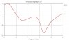
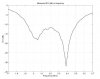
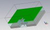
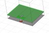
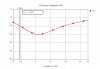
I'm new to CST microwave studio. Just finish constructed a structure of an L-probe patch antenna (from IEEE paper) and just run the simulation by transient time solver, the curve of the return loss(S11) against frequency that i get is different from what showing on the IEEE paper, so is it the boundary condition setting will affect the simulation results? And actually what is the function of setting the boundary condition?
During the simulation, a warning message "some PEC material is touching the boundary" was show. After change the boundary condition setting to "open(add space)" then the warning will eliminate when run again the simulation. But the s11 curve still different from the "actual" results.
Anybody can help?
Any comments will be appreciate.
Thanks.")
I'm new to CST microwave studio. Just finish constructed a structure of an L-probe patch antenna (from IEEE paper) and just run the simulation by transient time solver, the curve of the return loss(S11) against frequency that i get is different from what showing on the IEEE paper, so is it the boundary condition setting will affect the simulation results? And actually what is the function of setting the boundary condition?
During the simulation, a warning message "some PEC material is touching the boundary" was show. After change the boundary condition setting to "open(add space)" then the warning will eliminate when run again the simulation. But the s11 curve still different from the "actual" results.
Anybody can help?
Any comments will be appreciate.
Thanks.
Last edited: