Electro Tech is an online community (with over 170,000 members) who enjoy talking about and building electronic circuits, projects and gadgets. To participate you need to register. Registration is free. Click here to register now.
Welcome to our site! Electro Tech is an online community (with over 170,000 members) who enjoy talking about and building electronic circuits, projects and gadgets. To participate you need to register. Registration is free. Click here to register now.
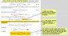
Q1: They are using p as a dummy integration variable so that it won't conflict with the s already used in the formula. The variables p and s are distinct. You often see dummy integration variables in time integrals too. Remember the use of tau in order to not conflict with the variable for time t.
Q2: They just mean that you can invert the integration order, as we typically do. I don't know what "uniform convergence" means, but personally I would proceed without worrying about it. This is a mathematical proof. As engineers we want to understand the gist of the proof, and we let the mathematicians worry about the rigor of the proof.
Q3: Yes, but G(s-p) is just G(s) with s replaced by (s-p). By the way, I hope you recognize that final formula as a convolution integral in the frequency domain. Basically, multiplication in the time domain transforms to convolution in the frequency domain, and convolution in the time domain transforms to multiplication in the frequency domain. These are very important properties to understand, and the duality/symmetry principle you see here is also an important concept in itself.
For Q1, the top version has either typos or mistakes right at the start of the work and the rest seems bad too. To see the mistakes, just compare to the other version. The bottom version seems closer to being correct, but still has a mistake because you have a tau in the result, but the tau=0, and then it is correct. Where did the top version come from?
Still, after the simple correction, the bottom version could do with some better precision in the notation. The functions you are convolving are t u(t) and exp(-3t) u(t), not t and exp(-3t). I know that we often get sloppy because single sided signals are implied, but one can make mistakes and readers might be confused if you are not clear. The starting integral is correct because the limits are chosen to reflect the u(t) functions, but I don't like this approach because it is not mathematically correct.
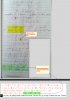
For Q2, why do you feel case 1 is not correct? Please explain. Also, what is the definition of the convolution integral and what are the limits of integration in the definition.
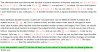
However, let's make an observation about case 1. In every step of case 1, it's clear that we are taking the inverse transform of G(s) which will yield g(t). This can be seen by inspection in every formulation. Clearly, G(s) (1) is G(s), and clearly g(t) * δ(t)= g(t)
For Q2, why do you feel case 1 is not correct? Please explain. Also, what is the definition of the convolution integral and what are the limits of integration in the definition.
However, let's make an observation about case 1. In every step of case 1, it's clear that we are taking the inverse transform of G(s) which will yield g(t). This can be seen by inspection in every formulation. Clearly, G(s) (1) is G(s), and clearly g(t) * δ(t)= g(t)
You should not have ended up with g(τ) because you integrated over the variable τ. When you integrate over a variable, that variable should disappear from the answer. In this case you will get g(t).
Unfortunately, you didn't try to answer the questions I posed. Hopefully, you at least thought about those questions. The definition of the convolution integral has limits from -∞ to +∞. You can argue that the lower limit is changed to 0 because the signal is single sided and thus is zero if t<0. But, why did you make the upper integral limit t? You need to think about this. In a general case, you can argue that the other signal you are convolving is also single sided, as so the upper limit must be t. However, let's be careful when that signal is an impulse function. Here we can first say the limits are -∞ to +∞, then we can say, the limits are 0 to +∞, and then we can say the limits are t- to t+, if we want to . Any and all of these give the same answer because the integral only has a contribution at the time t when the impulse is happening under the integral, and the sifting property of the delta function gives us the answer as g(t).
I'm sorry if it looked so. But I did understand what you were trying to point out and tried to correct my mistake, and this was the reason I changed the lower limit from 0 to 0-. But I think I should have tried to address the questions posted by you clearly; unfortunately I was (and am) really time pressed yesterday. Sorry.
So, I think you understand that your interpretation is correct.
Now, let's address your interesting question that you embedded in your comments. You said that when the input changes, the transfer function remains unchanged, and then asked "how?".
This is a another case when I give one of my (somewhat) annoying answers. The answer is, because that's the way we defined it to be.
If we don't narrow the scope of questions and problem down by making assumptions and restrictions, we can't make any headway. In this case, there is an entire theory based on linearity. A linear system has the property that the inputs don't change the transfer functions. Sometimes we make the additional assumption that the system is also time invariant, meaning that time does not change the transfer function. We call this an LTI (linear time-invariant) system. An LTI system has transfer functions that do not depend on time and do not depend on the input signals.
So, often our theory is limited to LTI systems, but real systems are almost never exactly an LTI system. Still, often the approximation is good enough. Component values may change over time, but the change might be slow. Transfer functions may depend on input signals, but over a limited range, the change may be small enough to neglect. etc. etc.
Always be careful if you try to apply Laplace theory to a nonlinear problem. The tool can be used via a linearization process, but there is always a risk that the nonlinearity is too strange or too severe to be amenable to analysis with that tool alone (or, at all).
This site uses cookies to help personalise content, tailor your experience and to keep you logged in if you register.
By continuing to use this site, you are consenting to our use of cookies.