simple integration problem: which answer is correct of the two, "0.5" or "-2"?

[PG1995]

Thank you, MrAl.

That function is exactly what you get when you substitute (t-3)/2 into the six equations we get from the original drawn function g1(t). It doesnt matter if it exceeds any other limit or equation because we dont integrate the whole thing, only part of it.

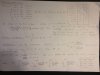
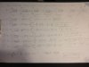
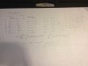
I think I have found my **broken link removed**. The point at t=3 in the graph in blue has been shifted to t=9 in red/pink graph because (0.5*9)-1.5=3. Please correct me if I'm wrong. Thanks.

Regards
PG

 

[MrAl]

Hi PG,

Well yes you're right that it is time scaled, but the two points you have there x and y are actually 4 units apart, not 3.5, so i think that saying that it is time shifted might not be the best way to look at it.
Because without the -1.5 the new graph would start at -1.5, but with the -1.5 it moves the first "zero crossing" of the entire ensemble, so maybe phase shifted (?) but that's loosely speaking too i guess. But yes it is time scaled.

You know how we get point y from x right? We do the 0.5*t-1.5 and get a value of -1 for t=x=1 so we look at the graph at t=-1 and we see that the point x is at -1, so we make the point at y equal to -1. Similarly, when we put the ordinate (7) into the equation we get '2' out, so we look up the value for what the original equation gives us at t=2, and we see that it is equal to 3, so we use 3 for the ordinate at 7 of the new plot.
So we use the ordinate from the calculation to "look up" the new value for that new ordinate using the new ordinate as the old ordinate to get the value and then using the new ordinate again to plot it. So it is:
1. old_x=0.5*new_x-1.5 (new_x is the x on the new graph where you want to plot the point)
2. Look up old_x on old graph, get old coordinate old_y.
3. Make new_y=old_y.
3. Go back to new_x on new graph, plot new_y as the point (new_x, new_y).


Another interesting point is that numerical integration works, but it doesnt seem to follow any of the methods we've used so far. The numerical solution requires ALL four of the first 'slopes', not just the first two like we've been doing so far. Skipping any of the four segments causes an incorrect result, and only using all four does it work. This means a piece by piece numerical integration works while an algebraic piece by piece doesnt work.
I havent figured out why yet. Interestingly, the first segment in the original plot integrates to a value of -1.9733333333... and that adds to the other three integrations so the whole adds up to exactly -3. Pretty amazing i think. I have the algorithm broken down so i can integrate each of the four sections independently, and then add up the results of all four.
I guess i'll have to look into this more at some point. Right now im working on some other things too which are ongoing daily.

 

[steveB]

Hi Steve,

Oh ok very good, thanks. That is the right result i believe. I would find it hard to believe that we could get two correct results using this method if it didnt work. What i was doing was searching for the limit of the method more or less.

How about one more, a little more tricky but lets see what happens...

Instead of g4=g1((t-3)/2) or the last, try using g4=g1((t^2-3/2). This is a non linear u this time.

OK, I worked this one out. It seems to work and I get 1.9732 as an approximate answer. I've attached 2 pages of work which also contains the exact answer. Then the 3rd page has a check of the answer using direct integration, with a Matlab programs to quickly handle the details.

I have to say that I would not normally have taken this substitution approach for this particular problem. Actually, the method I used to check the answer would have been my preferred approach, as that one only took a few minutes. The substitution method took me over an hour! However, it is useful to check it out and make sure the method is general. The method seems OK as far as I can tell.

The Matlab code to check the answer is as follows.

m=[-3 4 -3  1  3    1   ];
b=[9 -5  2  2  4    2   ];
p=[-sqrt(4.5)  -sqrt(3.5) -sqrt(2.5) -sqrt(1.5) -sqrt(0.5) sqrt(0.5) ];
q=[-sqrt(3.5)  -sqrt(2.5) -sqrt(1.5) -sqrt(0.5)  sqrt(0.5)    1      ];


for kk=1:6
    A(kk)=((m(kk)*q(kk)^3/3+(b(kk)-3*m(kk)/2)*q(kk))-(m(kk)*p(kk)^3/3+(b(kk)-3*m(kk)/2)*p(kk)));
end
sum(A)

 

[MrAl]

Hi Steve,

Wow, it looks like you really did a lot of work there. It wasnt my intention to have you do that much work i thought you would just throw the regular u substitution at it and see what we get, similar to before. Im not entirely sure what you actually did there, maybe you could explain it in words.

But did you at least try this numerically? Try that and compare results. I think you'll find a significant difference. Doing it numerically is quite easy if you have a program that integrates numerically. I checked the numerical solution against a raw graphical approach and the results agree quite closely, so i assume the two programs i used were correct because they both matched the raw graphical approach (which of course estimates the areas as a bunch of right triangles as you did previously). It's a bit harder with this one though because the remapping is not a bunch of straight lines but included curves too, but the curves are not too wild so it's not super difficult to estimate them as right triangles.

Would it help to view the remapping plot?

 

[steveB]

But did you at least try this numerically? Try that and compare results. I think you'll find a significant difference. Doing it numerically is quite easy if you have a program that integrates numerically.

I did it by two methods, and they both agree.

The first two pages use the substitution method. This does get complicated because of the nonlinear mapping.

The third page I just directly evaluate the integral, but I do it symbolically (with help from a Matlab program) rather than numerically.

Have you done it numerically and found a different result? If so, please tell me what number you are getting. If you are seeing a different answer numerically, then I will also do it numerically as a double check.

 

[steveB]

But did you at least try this numerically? ... Doing it numerically is quite easy if you have a program that integrates numerically.

I agree it is easy, and I used Matlab's mupad tool which has numerical integration built in. I've attached a screen-shot of the results and I get the same answer as the substitution method I worked out above.

In the screenshot, you will see that I defined the function using a piecewise description. Then I create a function f(t) . Then I numerically integrate the function f(t^2-3/2) over the range of t=-3 to t=1.

In the last line I enter the exact answer from the substitution method and I convert to a floating point approximation. It can be seen that the answers are equal to 10 decimal digits.

 

[MrAl]

Hi Steve,

Oh ok very good, thanks. That is the right result i believe. I would find it hard to believe that we could get two correct results using this method if it didnt work. What i was doing was searching for the limit of the method more or less.

How about one more, a little more tricky but lets see what happens...

Instead of g4=g1((t-3)/2) or the last, try using g4=g1((t^2-3/2). This is a non linear u this time.

Hi Steve,

Ok i see what happened now. You were doing t^2-3/2 and i was doing (t^2-3)/2 so we got different results.
If you look at the quote above you'll see:
g4=g1((t^2-3/2)
which is an incomplete statement because one close paren is missing.

Im sure if you did what i did you'd get the same results as i did, and if i did what you did i would get the same results as you did.

Now if you'd like to explain what you did in words that would be nice too
Originally all you did was use a simple u substitution, but this time you've done something else?
It's kind of hard to read those notes so it's hard to follow.

 

[steveB]

Now if you'd like to explain what you did in words that would be nice too
Originally all you did was use a simple u substitution, but this time you've done something else?

I can write up a general description of what I did in the next few minutes, but first let me be clear that I'm using the same basic method as before. The substitution is more involved because you gave me a harder problem. Also, whereas before I could add up the areas in my head and do the integration by inspection, this problem required that I actually write out the integrals for each region. So, it's much more work, more confusing and not as elegant in this case, but it's the same method.

As I mentioned above, I would not normally solve this harder problem using this technique. However, I view this exercise as a learning example for us to make sure the method is general and there is no unforeseen assumptions that must be valid for it to work.

 

[steveB]

Now if you'd like to explain what you did in words that would be nice too
Originally all you did was use a simple u substitution,

First of all, I am implementing a basic u=t^2-3/2 substitution. There are two things that make this tedious. First, the negative t-axis and the positive t-axis both map to the same u-values, so care is needed to get the formulation correct. Second, the piecewise nature of the function g1(t) requires careful determination of how t-values map to u-values and making sure the correct piece of g1 is used when integrating.

Page 1 Description:

The first page defines the function g1(t) as a piecewise function and then provides a table of domain-range, slope (m) and intercept (b) for each piece of the function.

Then an integral formula which is needed later is provided (note the formula is checked 3 ways to be sure it is correct)

Then the problem is stated as [latex] \int_{-3}^1 g_1(t^2-\frac{3}{2}) dt=A [/latex]

The problem is then solved with a direct u-substitution [latex] u=t^2-\frac{3}{2} [/latex]. There is then a problem determining "dt" because of the square root has two solutions (plus and minus values). So, the dt is defined as a piecewise function depending on whether t>0 or t<0. The new limits for u are then 7.5 to -1.5 as t goes from 3 to 1, but the section from u=-1.5 to u=-0.5 is traversed twice in the range of -1<t<+1. The integral as to be carefully written out and simplified as shown at the bottom of the first page.

Page 2 Description

The second page then simply works through the details of determining the written integral form. Each region of g1 has different "m" and "b" for the line function in that range. So, the integral needs to be broken into pieces, and it's clear that some of the range of "u" is where g1 equals zero. So, this entire page is just doing all the little area calculations. Then, all areas are added at the bottom to get the final answer. Note that the "exact" mathematical answer is given, and then an approximate numerical approximation is given.

Page 3 Description

The third page, does a direct symbolic calculation of the integral. I could have done an exact calculation here also, but I cheated and used a Matlab program to work out the math numerically and just provide direct verification that the answer on page 2 is correct. If page 3 is too confusing because of the compact notation, then just ignore that and use the numerical integration that I did in the follow on post. Basically, either method gives a numerical answer that validates the answer on page 2.

 

[MrAl]

Hi Steve,

Ok thanks, i'll have to look it over tomorrow sometime. In the mean time, PG can ask some questions about this last problem if he wants to.
I think it is informative to look at these kinds of problems.

 

[PG1995]

Hi

The following is text from MrAl's reply to this post of mine.

Well yes you're right that it is time scaled, but the two points you have there x and y are actually 4 units apart, not 3.5, so i think that saying that it is time shifted might not be the best way to look at it.

I have been thinking about it but couldn't get hold of it. It's true that there is an issue but I still can't see the reason why it isn't time shifted correctly. **broken link removed**, look at the two graphs for g1(t) and g4(t), the pink/red one is g4(t), you can see the problem MrAl pointed out.

g4(t) = g1( (t-3) /2 ) = g1( 0.5t -1.5 )

From the function expression above, it's easy to see that the function is time-scaled and then time-shifted. But what's the reason for the anomaly? Please help me with it. Thank you.

Regards
PG

 

[MrAl]

Hi,

See if this helps...

The red sine wave is at 2Hz and starts out at t= -0.5,while the blue sine is at 1Hz (1/2 frequency), but in order to get the blue wave to start out at the same place as the red wave (-0.5) we have to phase shift the blue wave by 180 degrees. This would appear as either an addition or a subtraction in the equation:
sin(w*t+180) or sin(w*t-180)

 

[PG1995]

q16, roberts

Hi

Could you please help me with this query, **broken link removed**.

If possible, please also help me with these queries, **broken link removed**. Thank you.

Regards
PG

 

[MrAl]

Hi there PG,


When you integrate two functions like this you get the sum of their areas. If area A was 1 and area B was 1 you get 1+1=2.
If one of the areas is negative, you end up adding two areas where one subtracts from the other, so if area A was 2 and area B was -1 you'd get 2-1=1.
Now you see a physical interpretation of where the constant of integration comes from in all of the indefinite integration formulas, like:
Integral(f'(t))=f(t)+C
That 'C' came from what happened before the current integration started.

To see this work in real life it isnt too hard using a circuit simulator. The pulses (or ramps) can be generated by current sources. The pulse is of course a current source that just takes on the values of the pulse amplitude for the required period of time, being negative if required.
The current source is then fed to a 1 Farad capacitor alone (no resistors) and the Integral of the pulse will be read as the voltage across the capacitor.
So for a pulse of amplitude 2 amps starting at t=0 and ending at t=1 we'll see the voltage rise as a ramp up to 2v, then if we change the pulse to -1 amp for t=1 to t=2 we'll see the voltage go down by 1v which leaves us with 1v at the end of 2 seconds.
If we use a pulse of 1 amp for t=0 to 1 and then a pulse of -1 amp from t=1 to 2 then the voltage will return to zero, but that's only because the second pulse had the negative area of the first pulse. We could have also applied a -1/2 amp pulse for 2 seconds (second pulse) to get back to zero volts across the cap.
Now if all of the signals are positive with none being negative, then the area will never go back to zero. The constant of integration for the second pulse comes from the value of the integral (the voltage across the cap) at the very end of the previous pulse, so that gets added to the new integral over the new pulse period.
So the second g(t) you have there does not ever integrate to zero because there is never any negative area to cancel out the positive areas.
Another way to think of it is the final result is the sum of the positive areas minus the absolute value of the sum of the negative areas.
It's actually becomes very simple when you do a few of these.
Also, if you parameterize each ramp in your second g(t) you'll find that when you integrate both over the periods you have to do:
Integral[0 to 1](g1(t)) dt + Integral[1 to 2](g2(t)) dt
so you are just summing the parts.

The rect() function shown in your second note is not the best representation of that function. The better representation is
rect(x)=a for |t|<1/(2*a)
so we can control the amplitude.
This function 'rect' is an area function where we think of the bulk of the pulse being at zero. If we think about it, it's called 'rect' and that stands for 'rectangular', but why would we have to call a function of x (like y=f(x)) by a name that stands for something that describes something with an area.
So see if that makes any more sense.
If you integrate a regular pulse that starts at t= -1/2 and ends at t= +1/2 and has a height of 1, you get an area of 1, and the area passed (accumulated) by the time we get to t=0 is 1/2, so if it was just an ordinary pulse we'd get Integral(g(t)) dt = t+0.5.

BTW, where is the reference that told you that Integral(rect(t))dt=t ?

Perhaps Steve would care to chime in on this too.

 

[steveB]

PG,

When I look at your comments, I feel that there must be an underlying misconception that has generated this series of questions. I think our first task is to identify this misconception, and I'm going to take a guess at what it might be.

As I read what you wrote, I wonder if you are forgetting that there are two different meanings of integration.

First, there is the idea of an "anti-derivative". If we have a function like y=x^2, we know the derivative is dy/dx=2x. The anti-derivative of 2x is then x^2 + C. Notice that when we reverse the operation, we need to add a constant C because the derivative of a constant is zero, and so any value of C provides a valid anti-derivative. We also call the anti-derivative operation an "indefinite integral". When you look at a table of indefinite integrals, you might see the following, although sometimes the constant C is left out because it is known to always be present.

[latex]\int x\;dx=\frac{x^2}{2}+C[/latex]

Second, there is the idea of a "definite integral" and this is the idea of area under a curve. Here, we must specify two limits for the integration, and the constant C is not relevant because it will subtract out. Let's do a simple definite integral of y=x over the range of 0 to 1. Clearly, we know the answer is 1/2 just by looking at the graph, but let's do it formally and notice how any constant C gives the same answer because it subtracts out. Since is always subtracts out, it is traditional to use C=0 when doing definite integrals.

[latex]\int_0^1 x\; dx=\left[\frac{x^2}{2}+C \right] _0^1=(\frac{1^2}{2}+C)-(\frac{0^2}{2}+C)=\frac{1}{2}[/latex]

Now, how does this relate to your questions?

For question Q, notice that your question 14 says to integrate from negative infinity to some value of "t". This implies a definite integral over a range, and the area is the cumulative area under the curve from negative infinity to a particular point. Let's write this integral out formally and notice the use of a dummy integration variable tau.

[latex]h(t)=\int_{-\infty}^t g(\tau)\; d\tau[/latex]

Notice that even though the function is g(t), we put it in the integral as a function of tau and integrate over the variable tau. Here, tau is a dummy integration variable that goes away after the operation, and you are left with a new function of "t", which I called h(t) above.

The meaning of h(t) is the area under the curve g(t) from negative infinity up to the point "t". So, this is why the area can't be zero in your example when t>2.

Now, what about Q1? This is a bit of a silly question, but I realize you are just trying to rationalize how to get a particular result. We never make area negative just because t<0.

Now, for Q2. Hopefully, my above description of area being a definite integral answers this. You can't just say the area for the rect(t) function is "t" and therefore the area at t=0 is zero. No, you have to do out a full definite integral with proper limits to get area.

So, let's do it out. First, rect(t)= zero for t<1/2, so instead of starting the integration at negative infinity, we can start at -1/2. All area up to t=-1/2 is zero.

[latex]A=\int_{\frac{-1}{2}}^t {\mathrm {rect}}(\tau)\; d\tau=\left[t\right] _{\frac{-1}{2}}^t={t}+\frac{1}{2}[/latex] for -1/2<t<1/2, and A=1 for t>1/2 and A=0 for t<-1/2

Notice that I restrict this answer t+1/2 to be for -1/2<t<1/2 because the "rect" function goes to zero outside this range and the antiderivative is zero (strictly it is any constant number, but it subtracts out) there. Clearly, the area is one for t>1/2. You can see this visually in the plot, or you can do it formally with definite integrals.

 

[PG1995]

Thank you, MrAl, Steve.

@Steve: Yes, you are right. I did have a confusion about antiderivative and definite integral somewhere in my mind although I didn't realize it before! But worse thing is confusion has begged more confusion. Now please help me with these queries, **broken link removed**, and **broken link removed**. Thanks a lot.

Regards
PG

 

[steveB]

Thank you, MrAl, Steve.

@Steve: Yes, you are right. I did have a confusion about antiderivative and definite integral somewhere in my mind although I didn't realize it before! But worse thing is confusion has begged more confusion. Now please help me with these queries, **broken link removed**, and **broken link removed**. Thanks a lot.

Regards
PG

For Q1: I think we may be talking about different things. In your original question, you asked if "we also take area to be negative for negative values of the independent variable, even when the function's value is positive". To me this means you are asking if the area would be negative automatically when t<0, which is NOT true. Area is simply not defined this way. However, any area below the t-axis is considered negative. Perhaps this is what you are really asking, in which case, yes is the answer. Wording is very important in a question.

For Q2: I think the text is OK. This is just a confusing point and the author does not find the clearest way to express it.

For Q3: The point of where you want to start integrating is arbitrary. Take it to be negative infinity if you like. Basically, the starting point and the addition of the constant are the same thing. You have to spend some time thinking about it and sketching out a few examples to get comfortable about this idea.

 

[PG1995]

Thank you, Steve.

I have **broken link removed** from my previous post. You can also see the attachment in PDF format here. I would suggest that you first have a look on my previous post to refresh your memory about what was being discussed there. Thanks a lot.

Regards
PG

 

[steveB]

For Q1, I would say that you are not allowed to make up your own rules. Why are you arbitrarily assigning negative width to the negative side of the x-axis? This is not how the width is defined. We define integration to be from the limit on the bottom to the limit on the top. This means that the width will have the same sign on either side of the x=0 on the x-axis.

For Q2, i just don't understand what your concern is. Is there a concept you are trying to make sure you understand correctly? If so, then just try to state the question independent of the book. We don't always need to refer to a book to answer a question, and neither one of us are in the business or criticizing books and providing editorial feedback to the authors.

For Q3, yes, you make sense. We dont' need the constant when we do definite integrals because any constant we choose will subtract out. I stressed this point earlier, and said that the usual convention is to assume C=0 when doing definite integrals. I assume you understand that finding area is an example of a definite integral.

 

[PG1995]

1.1 (Q8), Burden

Hi

Could you please help me with **broken link removed** query? Thanks a lot.

Regards
PG